Forecasting Brazilian aquaculture production using multivariate analysis and time-series models


Pronóstico de la producción acuícola brasileña mediante análisis multivariante y modelos de series temporales


Murilo Henrique Tank Fortunato¹*; Karoline Moreira Barbuio²; Juliana Antunes Galvão³; Wagner Dos Anjos Carvalho1 


1 MBA USP/ESALQ, R. Cezira Giovanoni Moretti, Piracicaba, Brasil.

2  Departamento de Ciencia Animal, Avenida Pádua Dias, 11, barrio Agronomía, Piracicaba, Brasil.

3  Departamento de Ciencia de los Alimentos, Avenida Pádua Dias, 11, barrio Agronomía, Piracicaba, Brasil.


ORCID de los autores:

M. H. Tank Fortunato: https://orcid.org/0000-0002-1695-8120 K. M. Barbuio: https://orcid.org/0009-0002-1467-4092

J. A. Galvão: https://orcid.org/0000-0003-4222-6801  C. dos A. Carvalho: https://orcid.org/0000-0003-2754-4414


RESUMEN


Este estudio analizó la producción acuícola brasileña entre 2013 y 2023, con énfasis en la tilapia, el tambaqui y el camarón, utilizando datos oficiales del Instituto Brasileño de Geografía y Estadística (IBGE). El Análisis de Componentes Principales (ACP) y el algoritmo de agrupamiento PAM identificaron tres perfiles regionales de producción: la región Sur, asociada principalmente al cultivo de tilapia; la región Nordeste, especializada en la producción de camarón; y un tercer grupo, integrado por las regiones Norte, Centro-Oeste y Sudeste, caracterizado por una producción diversificada. Los resultados evidenciaron el fuerte crecimiento de la tilapia, consolidando su liderazgo en la acuicultura brasileña. Se evaluaron modelos predictivos, incluyendo Regresión Lineal, ARIMA y Random Forest, mediante el Error Absoluto Medio (MAE). El modelo ARIMA presentó el mejor desempeño al capturar los patrones temporales y proyectó un crecimiento continuo de la producción de tilapia hasta 2030, mientras que el tambaqui y el camarón mostraron una tendencia de estabilidad. Entre las limitaciones del estudio se encuentra el uso de datos anuales agregados, que pueden no reflejar cambios recientes en el sector. Los hallazgos proporcionan información relevante para apoyar la planificación estratégica y el desarrollo de políticas públicas orientadas al fortalecimiento de la acuicultura.


Palabras clave: producción acuícola; cultivo de tilapia; pronóstico mediante ARIMA; análisis de componentes principales; Brasil; economía acuícola.


ABSTRACT


This study analyzed Brazilian aquaculture production between 2013 and 2023, focusing on tilapia, tambaqui, and shrimp, using official data from the Brazilian Institute of Geography and Statistics (IBGE). Principal Component Analysis (PCA) and PAM clustering identified three regional production profiles: the South, associated with tilapia farming; the Northeast, specialized in shrimp; and a third group (North, Central-West, and Southeast) with diversified production. Results highlight the strong growth of tilapia, consolidating its dominance in Brazilian aquaculture. Predictive models, including Linear Regression, ARIMA, and Random Forest, were evaluated using Mean Absolute Error (MAE). ARIMA showed the best performance, capturing temporal patterns and projecting continued tilapia growth until 2030, with stability for other species. Limitations include the use of aggregated annual data, which may not capture recent sectoral changes. The findings support planning and policy development in aquaculture.


Keywords: aquaculture production; tilapia farming; ARIMA forecasting; principal component analysis; Brazil; aquaculture economics.


  1. Introduction

Aquaculture, understood as the cultivation of aquatic organisms in controlled environments, has become one of the pillars of global food security throughout the 21st century. The continuous growth in demand for high–biological-value protein, combined with the stagnation of capture fisheries at sustainable production levels, has driven aquaculture to assume a central role in the supply of aquatic foods. According to the Food and Agriculture Organization of the United Nations (FAO, 2024), aquaculture production has already surpassed capture fisheries as the main source of fish for human consumption, standing out for its high feed conversion efficiency, potential for large-scale production, and adaptability to diverse socio-environmental contexts.

In Brazil, this expansion scenario is particularly evident. The country benefits from favorable edaphoclimatic conditions, abundant water resources, an extensive coastline, and large hydrographic basins, all of which support the growth of national aquaculture. According to data from the Brazilian Fish Farming Association (Peixe BR, 2025), tilapia farming leads Brazilian aquaculture production, consolidating itself as the sector’s main segment. At the same time, shrimp farming and the cultivation of native species, such as tambaqui (Colossoma macropomum), play a strategic role, especially in specific regions of the country. Despite the progress achieved, the FAO (2024) emphasizes that Brazil, although ranked among the largest aquaculture producers in Latin America, still has significant underexploited productive potential.

In this context, the use of data analysis tools has become increasingly relevant to the sustainable development of aquaculture. The growing availability of information on production, markets, and environmental variables enables the application of statistical and machine-learning methods capable of identifying patterns, modeling complex relationships, and supporting decision-making processes (Presenza et al., 2025). Time-series models, such as ARIMA, are widely employed to capture trends, seasonality, and autocorrelation structures in longitudinal data (Box et al., 2015; Panagiotelis et al., 2021).

Additionally, linear regression methods and tree-based algorithms, such as Random Forest, stand out for their robustness in modeling nonlinear relationships and handling high-dimensional datasets (Biau & Scornet, 2016). Multivariate approaches, such as Principal Component Analysis (PCA), allow for dimensionality reduction and the identification of dominant patterns of variability (Jolliffe & Cadima, 2016), while clustering techniques, such as the Partitioning Around Medoids (PAM) method, enable the segmentation of regions or production systems based on similar characteristics (Kaufman & Rousseeuw, 2009).

Thus, the integrated application of these statistical and computational tools goes beyond mere scenario forecasting, contributing to strategic planning, sustainable aquaculture management, and the formulation of evidence-based public policies.

In light of this framework, the present study aims to analyze the evolution of Brazilian aquaculture production between 2013 and 2023, with emphasis on the main farmed species, tilapia, tambaqui, and shrimp, identify regional patterns of productive specialization, and project prospective scenarios through 2030.

We hypothesized that Brazilian aquaculture exhibits distinct regional production patterns and that time-series models, particularly ARIMA, provide more accurate forecasts than traditional regression and machine-learning approaches.


2. Methodology


The analytical procedure was conducted using the R programming language, employing a set of statistical and data-manipulation packages to ensure the robustness and integrity of the analysis. The study adopted a quantitative approach, with a methodological focus on exploratory analysis of secondary data. The database was obtained from the Brazilian Institute of Geography and Statistics (IBGE) and contains annual aquaculture production data (kg) covering the period from 2013 to 2023 (https://sidra.ibge.gov.br/tabela/3940).

After exporting the original data in CSV format, a tabulation and filtering stage was performed, in which the 20 most representative and relevant species in national production were selected. These data were organized into a new file, named Aquicultura.csv, which served as the structured basis for subsequent analyses.

During the preprocessing stage, the absence of production records for a given species in a specific region was not treated as random missing data; but rather interpreted as an indication of non-production. This pattern falls under the category of Missing Not at Random (MNAR), according to the typology proposed by Little and Rubin (2002), thereby justifying the assumption that “not reported” values correspond to zero production. Accordingly, to ensure that the analysis reflected only actual production, null records were excluded, retaining only observations with Producao_kg > 0.

Data standardization was carried out by harmonizing variable nomenclature to Region, Year, Species, and Production_kg, as well as by converting numerical values to the appropriate format.

Following data tabulation and preprocessing, initial descriptive analyses were conducted, followed by the application of Principal Component Analysis (PCA) to reduce data dimensionality and facilitate the interpretation of underlying patterns. In the segmentation stage, clustering was performed using the Partitioning Around Medoids (PAM) method, with the elbow and silhouette criteria applied to determine the optimal number of clusters. Finally, predictive models, including ARIMA, decision trees, and linear regression, were implemented to model and forecast the behavior of the analyzed variables (Kaufman & Rousseeuw, 2009; Jolliffe & Cadima, 2016; Box et al., 2015; Biau & Scornet, 2016).

The analyses were supported by statistical packages such as tidyverse, readr, reshape2, and lubridate for data acquisition and preprocessing; forecast, e1071, caret, and randomForest for predictive modeling; and cluster, factoextra, and corrplot for clustering and principal component analyses. All code developed for this study is publicly available at: https://github.com/mtank6691-coder/C-digo-TCC-Murilo-/blob/main/DATA%20SCIENCE%20MURILO%20TANK.


2.1 Exploratory Data Analysis (EDA)

Exploratory Data Analysis (EDA) was conducted with the purpose of statistically describing the dataset and guiding the formulation of hypotheses to be tested in subsequent stages of predictive modeling. For this purpose, the ggplot2 library was employed.

Among the visualizations produced, bar charts representing total production by region and by species stand out. Categories were ordered in descending order based on production volume using the reorder() function. The choice of this type of chart is grounded in its effectiveness in representing categorical variables with numerical aggregations, as discussed by Cleveland (1985) in his work on best practices in data visualization.


2.2 Principal Component Analysis (PCA)

Principal Component Analysis (PCA) is a statisti-cal technique widely used for dimensionality reduction, whose objective is to transform a set of correlated variables into a new set of orthogonal (uncorrelated) variables, known as principal com-ponents (Jolliffe & Cadima, 2016). Its application in this study is justified by the need to extract the main variance structures from the data and to identify associations between regions and aqua-culture species based on their production profiles.

Mathematically, the first principal component (PC1) is defined as a linear combination of the original variablesnX_1,X_2,…,X_p , expressed as:

PC1=a11X1+a12X2 +⋯+a1p Xp x'

where the coefficients a_1jcorrespond to the elements of the eigenvector associated with the largest eigenvalue of the covariance (or correlation) matrix and represent the contribution of the variable X_jto the formation of the principal component. These eigenvectors indicate the directions of maximum variance in the multivariate data space (Jolliffe & Cadima, 2016). The second principal component (PC2) is also a linear combination of the original variables, given by:

PC2=a21X1+a22X2+⋯+a2p Xp

being defined based on the eigenvector asso-ciated with the second largest eigenvalue of the covariance or correlation matrix. PC2 is orthogonal to PC1 and explains the largest possible proportion of the remaining variance not captured by the first component. Thus, while PC1 represents the primary gradient of variation in the data, PC2 reveals secondary patterns of differentiation among observations, contributing to a more in-depth understanding of the associations between regions and aquaculture species.

To prevent variables with larger numerical magnitudes from disproportionately influencing the PCA results, the data were previously standardized using the function prcomp (..., scale. = TRUE), ensuring that all variables had a mean of zero and a standard deviation of one (Rencher & Christensen, 2012). Standardization is particu-larly important when variables are measured on different scales, which is common in studies involving production data.

The interpretation of the results was enhanced using the factoextra package, which provides effective visualization tools for principal compo-nent analysis. The plots generated using the fviz_pca_ind() function enabled the visualization of similarity patterns among regions (Kassambara, 2017).

2.3 Clustering analysis

To group regions based on similar production profiles, a clustering approach centered on the Partitioning Around Medoids (PAM) method was employed. This technique was chosen due to its greater robustness to the presence of outliers when compared to the traditional K-means algorithm. While K-means relies on centroids, hypothetical mean values that may not correspond to actual observations, PAM operates with medoids, which are real data points from the dataset and therefore more accurately represent the central elements of each group (Kaufman & Rousseeuw, 2009).

The PAM algorithm functions by minimizing the sum of dissimilarities between each observation and the medoid of the cluster to which it belongs. To compute these dissimilarities, the Euclidean distance was used, defined by the following mathematical expression:
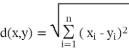
where x and y represent vectors of observations and n denotes the number of variables conside-red. This metric allows quantifying the degree of similarity (or dissimilarity) between two regions based on their production profiles.

The determination of the optimal number of clusters (k) was performed and validated using internal statistical validation methods, notably the Elbow Method and Silhouette Analysis. The Elbow Method consists of evaluating the variation in the sum of intra-cluster dissimilarities as a function of the number of clusters, with the optimal number of groups identified at the point where a less pronounced marginal reduction in this measure occurs, characterizing an “elbow” in the curve.

Complementarily, Silhouette Analysis was emplo-yed to assess clustering quality based on intra-cluster cohesion and inter-cluster separation. The silhouette coefficient for an observation i is given by:
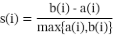
where a(i)represents the average distance from observation i to all other observations belonging to the same cluster, and b(i)corresponds to the smallest average distance from i to observations in any other cluster. The value of s(i)ranges from −1 to 1, with values close to 1 indicating an appropriate assignment of the observation to its cluster and good separation from the remaining clusters, thus evidencing a satisfactory clustering configuration.

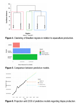
Complementary to the PAM partitioning technique, a Hierarchical Clustering Analysis was conducted in order to explore the hierarchical structure of the groupings in a visual and intuitive manner. The Ward.D2 linkage method was applied, which seeks to minimize total within-cluster variance at each step of cluster fusion. Euclidean distance was likewise adopted as the dissimilarity metric.

The results of this analysis were represented through a dendrogram, allowing the visualization of similarity relationships among fish-producing regions at different levels of aggregation and serving as a complementary tool for the inter-pretation and validation of the clusters obtained.


2.4 Predictive modeling methodology

The final phase of this study focused on the application and comparison of three predictive modeling approaches aimed at forecasting the future production of the main aquaculture species. The use of multiple models, combined with the application of formal performance evaluation crite-ria, ensured greater robustness of the generated estimates and enabled a comprehensive compa-rative analysis of the adopted methodologies.


2.5 Performance metric and validation strategy

To assess model accuracy, the Mean Absolute Error (MAE) was adopted as the performance metric. This measure was selected due to its interpretability, as its values are expressed in the same unit as the original data (kg), thereby facilitating direct comparison between observed and predicted values (Hyndman & Koehler, 2006).

The MAE is formally defined as:
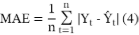
where Y_trepresents the actual production value at observation t, Y ̂_tcorresponds to the value predicted by the model for the same observation, and ndenotes the total number of observations considered.


2.6 Training and testing strategy

The evaluation and forecasting methodology was based on predictive time-series analysis. The historical dataset covering the period from 2013 to 2022 was used as the training set, while data for the year 2023 were reserved as the test set. This strategy ensures an unbiased assessment of the models, as the validation data were not used during the training process (Hyndman & Athanasopoulos, 2018).

Because the time series consisted of only eleven annual observations, more complex resampling strategies, such as repeated cross-validation or rolling-origin evaluation, were not considered appropriate. Under these circumstances, the hold-out approach represents a robust and widely accepted validation strategy for short annual time series. The same train-test split approach, as well as performance comparison, was consistently applied to both the total production series and the species-specific production time series.


2.7 Evaluated predictive models

Three distinct predictive models were evaluated for each analyzed time series (total production and species-specific production): Linear Regression (LM), Random Forest (RF), and ARIMA.


2.8 Linear Regression (LM)

The first model evaluated was Linear Regression (LM), a classical statistical model that assumes a linear relationship between the response variable (production) and the explanatory variable time (year). Its main advantage lies in its ease of implementation and interpretability. However, its fundamental limitation is the inability to capture more complex patterns, such as nonlinear behaviors or structural changes, which are frequently observed in economic and production data (Box et al., 2015).


2.9 Random Forest (RF)

The second model considered was Random Forest (RF), a machine-learning technique based on an ensemble of decision trees, where the aggregation of individual predictions contributes to increased robustness and predictive power (Biau & Scornet, 2016). This model was included to capture nonlinear relationships present in the data. To mitigate the risk of overfitting, five-fold cross-validation was employed using the trainControl function. This strategy ensured that the model was evaluated across different subsets of the training data, promoting greater generalization of predictions.


2.10 ARIMA (AutoRegressive Integrated Moving Average)

The third model evaluated was ARIMA, widely used in time-series analysis due to its ability to capture trends, seasonal patterns, and autoco-rrelations, that is, the dependence between present and past values of the series (Shumway & Stoffer, 2017).

An ARIMA model is denoted as ARIMA(p, d, q), combining three fundamental components: autoregressive (AR), integration (I), and moving average (MA). Its general formulation is expressed as:

(1-ϕ_1 B-…-ϕ_p B^p)(1-B)^d Y_t=c+(1+θ_1 B+⋯+θ_q B^q)ε_t (5)

The term Y_trepresents the value of the time series at time t; ϕ_iare the autoregressive parameters; θ_iare the moving average parameters; dcorresponds to the number of differences applied to the series to achieve stationarity; Bis the backshift (lag) operator; and ε_tis the random error term, assumed to be white noise.

The auto.arima() function from the R forecast package was used to automatically select the optimal values of pand q, based on information criteria such as the Akaike Information Criterion (AIC) and the Bayesian Information Criterion (BIC). This approach allowed the fitting of models tailored to the dynamic characteristics of each individual production time series, following the methodology described Hyndman & Athanasopoulos (2018).

2.11 Forecasting Strategy and Scope of Analyses

Among the models evaluated for the total production series, ARIMA exhibited the best performance according to the MAE and was therefore selected as the reference model for supporting the final conclusions of the study.

However, for the production series of the key species, forecasts were generated using all three models (LM, RF, and ARIMA), with the objective of enabling a comparative analysis between linear, nonlinear, and time-series–specific approaches. Projections were made for a seven-year horizon (2024–2030), covering the following categories:

    Tilapia: the species with the highest production volume;

    Tambaqui: one of the main native species;

    Shrimp: representative of shrimp farming;

    Oysters, scallops, and mussels: a group characterized by high added value.

3. Results and discussion

3.1 Exploratory analysis

The exploratory analysis of the data revealed a significant growth in Brazilian aquaculture over the last decade, with annual production increasing from approximately 484,000 tons in 2013 to over 887,000 tons in 2023. However, this production (Figure 1A) is not evenly distributed across the country, being concentrated primarily in key regions such as the South, followed by the Northeast and Southeast. This regional predomi-nance is explained by factors such as favorable climatic conditions, developed infrastructure, and historical investment in the sector. Additionally, production is dominated by a few species, Figure 1B, with Tilapia, Tambaqui, and Shrimp accoun-ting for the majority of total output.

Principal Component Analysis (PCA) was applied to identify latent patterns and group regions with similar production characteristics, Figure 2.A. Native species such as Tambaqui, Pirarucu (Arapaima gigas), and Matrinxã (Brycon amazonicus) are concentrated in the North and Central-West regions, reflecting the relationship between local biodiversity and regional production potential. These species are adapted to the ecological conditions of the Amazonian and Pantanal rivers, favoring their adoption as production focuses. The Northeast shows a predominance of Shrimp, consolidating shrimp farming as a strategic activity due to the limitation of inland water resources. Meanwhile, the South and Southeast cluster around Tilapia, highlighting historical investments in intensive systems, infrastructure, and specific incentive policies.

The analysis of species’ contributions to the principal components shows that Dim1 explains 48.4% of the data variability, while Dim2 explains 24.7%, totaling approximately 73%. Species such as Tilapia, Traíra, and Trairão are strongly associated with the positive Dim1 axis, indicating intensive and consolidated production systems (Figure 2B).
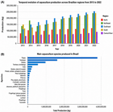
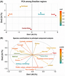
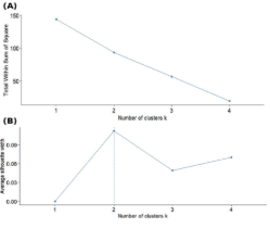


Figure 1. A. Temporal evolution of aquaculture production across Brazilian regions from 2013 to 2023. B. Main aquaculture species produced in Brazil.

Figure 2. A. PCA among Brazilian regions. B. Species contributions to principal component analysis.


3.2 Principal Component Analysis (PCA)

Conversely, Tambaqui, Pirarucu, Curimatã (Prochilodus lineatus), and Tucunaré (Cichla ocellaris) are associated with the negative Dim1 axis, reflecting production systems more linked to native species and specific to the North and Central-West regions.

The Dim2 axis separates Shrimp, strongly associated with the positive direction of the component, indicating a distinct production pattern, while Pacu (Piaractus mesopotamicus), Patinga (hybrid), and other round-fish groups appear in the negative direction, representing another production pattern. The angular proximity between arrows indicates positive correlation, while opposite directions reflect distinct production patterns. Thus, PCA highlights production gra-dients and the species that structure Brazilian aquaculture.

3.3 Elbow Method and Silhouette Analysis

The elbow method was used to determine the optimal number of clusters in the clustering, Figure 3.A, analysis by examining the within-cluster sum of squares (WSS) as a function of the number of clusters. The curve indicates that three clusters represent the ideal point, as the reduction in WSS becomes less pronounced beyond this point, showing that adding more clusters does not significantly improve group compactness.

Silhouette analysis, which evaluates the cohesion within clusters and the separation between clusters using coefficients ranging from -1 to 1, suggests an inflection point at two clusters. Higher silhouette values indicate more clearly defined and well-separated clusters, while lower or negative values may signal overlapping or poorly defined groupings. This analysis provides a complemen-tary assessment of the elbow method, reinforcing the selection of the optimal number of clusters by not only considering the reduction in within-cluster variance but also the quality and distinctiveness of the clusters identified (Figure 3B).


3.4 Clustering results

Clustering of regions based on the similarity of production profiles confirms the patterns observed in the PCA (Figure 4). The clusters reveal that the North and Central-West regions are distinguished by the production of native species such as Tambaqui and Pirarucu; the Northeast is characterized by Shrimp; and the Southeast and South share production profiles with Tilapia as the key species. The high contribution of Tilapia, Tambaqui, and Shrimp to variability is determinant in forming these groups.


3.5 Predictive analysis

The accuracy of predictive models was evaluated using the Mean Absolute Error (MAE), representing the average absolute differences between predicted and observed values in kilograms for 2023 (Figure 5). ARIMA showed the lowest mean absolute error, with an MAE of 19,825,195.67 kg, indicating an average deviation of approximately 19.8 million kg. Linear Regression recorded an MAE of 61,592,312.47 kg, and Random Forest presented an MAE of 92,433,430.94 kg. Despite ARIMA’s better overall performance, Linear Regression and Random Forest were applied by species to capture distinct production patterns.

ARIMA excels at capturing temporal dependence and structural variations. Linear Regression allows for interpretation of average trends, while Random Forest showed limitations in short time series, reproducing mean values without extrapolating trends.


3.6 Projections by Species

Tilapia projections up to 2030 indicate continuous growth (Figure 6) according to ARIMA, reaching approximately 633 million kg. Linear Regression shows steeper growth over the period, while Random Forest maintains nearly constant projections. For 2024, ARIMA estimates 469,000 tons, whereas PeixeBR data indicates about 662,000 tons, reflecting lags in the IBGE historical series and recent structural changes, such as domestic market expansion, exports, and greater professionalization of the production chain.


Figure 3. A. Elbow graph. B. Silhouette graph.


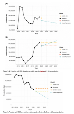
For Tambaqui and Shrimp, ARIMA projects maintenance, of recent observed values until 2030, estimating 111.5 million kg for Tambaqui and 127.5 million kg for Shrimp. Linear Regression indicates slight decline for Tambaqui and growth for Shrimp, reflecting average trends, while Random Forest maintains constant values, limited by the absence of additional temporal variables (Figure 7).

The group of Oysters, Scallops, and Mussels shows production stability, with ARIMA projecting 8,729,164 kg in 2024, remaining constant until 2030. Linear Regression suggests a slight decline, and Random Forest values remain close to the last observed. Despite statistical stability, the sector is heavily concentrated in Santa Catarina, which accounts for over 95% of national production, making it sensitive to environmental and sanitary shocks (Figure 8).

The exploratory analysis confirmed the significant expansion of Brazilian aquaculture over the past decade, reflecting a broader global trend in which aquaculture has become one of the fastest-growing food production sectors. As capture fisheries approach biological limits in many regions, aquaculture has increasingly assumed a central role in supplying animal protein and supporting global food security (FAO, 2024).

In Brazil, favorable environmental conditions, abundant freshwater resources, and increasing technological adoption have enabled the consolidation of aquaculture as a strategic component of the national agrifood system (Carneiro, 2022). Recent sectoral reports also indicate a consistent expansion of Brazilian aquaculture production, particularly in tilapia farming and shrimp production (Peixe BR, 2025; ABCC, 2025).


Despite this growth, production remains geogra-phically and taxonomically concentrated. The South, Northeast, and Southeast regions dominate national production, largely due to infrastructure availability, historical investment, and technological development in aquaculture systems. Similar patterns of regional specialization have been documented in several aquaculture-producing countries, where climatic suitability, logistics, and market access influence the spatial distribution of production systems. The dominance of a limited number of species, particularly tilapia, tambaqui, and shrimp, reflects the biological and economic advantages of these species, including high growth rates, established production technologies, and strong market demand.

The multivariate analysis provided additional insight into the structural organization of Brazilian aquaculture production. The PCA results revealed clear regional production patterns, highlighting the role of ecological and economic factors in shaping species distribution. Native Amazonian species such as tambaqui and pirarucu remain concentrated in the North and Central-West regions, reflecting their adaptation to local environmental conditions and river basin characteristics (de Fátima Vidal, 2022). In contrast, shrimp farming predominates in the Northeast due to favorable coastal environments and saline water availability. The South and Southeast regions are strongly associated with tilapia production, reflecting long-term investments in intensive farming systems, genetic improvement, and integrated production chains (Carneiro, 2022).

The clustering analysis corroborated regional production patterns identified through PCA. By grouping regions according to production similarity, the analysis demonstrated that Brazilian aquaculture operates through distinct regional production systems. Such analytical approaches have been increasingly applied in aquaculture studies to identify production clusters, optimize resource allocation, and support regional development strategies within the sector.

From a methodological perspective, the use of predictive modeling represents an important contribution to this study. Aquaculture production systems are influenced by complex interactions among environmental conditions, market forces, technological innovation, and policy interventions. Consequently, forecasting techniques such as ARIMA, linear regression, and machine learning models have increasingly been applied to fisheries and aquaculture datasets to identify production trends and support decision-making processes.

The superior performance of the ARIMA model in the aggregated analysis aligns with previous studies demonstrating that time-series models are effective for capturing temporal dependence and structural trends in aquaculture production data. ARIMA-based approaches have been widely used to forecast fisheries and aquaculture outputs, providing insights into production variability and supporting strategic planning in the sector (Nabi et al., 2025). However, when the analysis was conducted at the species level, different models showed distinct performances. In some cases, linear regression captured production trends more effectively, particularly when the underlying pattern followed a relatively stable linear trajectory over time. This finding highlights the importance of evaluating multiple modeling approaches when forecasting aquaculture production, as different species and production systems may exhibit distinct temporal dynamics.

The integration of statistical modeling and data science approaches is becoming increasingly relevant in modern aquaculture. Data analytics enables researchers and policymakers to transform large volumes of production data into actionable information, improving resource management, production efficiency, and long-term planning (Lukambagire et al., 2023). Recent studies also emphasize the growing role of machine learning and artificial intelligence in aquaculture management, including production forecasting, environmental monitoring, and decision support systems (Rather et al., 2024; Hu et al., 2025). The emergence of precision aquaculture illustrates how digital technologies can enhance productivity while maintaining environmental sustainability.

Nevertheless, limitations associated with official production statistics must be acknowledged. National datasets such as those produced by IBGE provide consistent long-term information but may not fully capture short-term structural changes occurring within the sector. Similar limitations have been identified in aquaculture statistical systems in other countries, where discrepancies between official records and field observations may influence the interpretation of production trends (Abdel-Hady et al., 2025). In the Brazilian context, recent industry reports suggest that sector growth, particularly in tilapia and shrimp production, may be more dynamic than indicated by official annual statistics (Peixe BR, 2025; ABCC, 2023).

Overall, the findings demonstrate that Brazilian aquaculture development is shaped by a combi-nation of ecological conditions, technological investments, and market dynamics. The integra-tion of multivariate statistical analysis with predictive modeling provides a robust analytical framework for understanding the spatial organi-zation and temporal evolution of aquaculture production systems. As the sector continues to expand globally, the incorporation of advanced data science techniques, including machine learning, artificial intelligence, and big data analytics, will become increasingly important for supporting sustainable aquaculture management and evidence-based policy formulation.


4. Conclusions

The results of this study highlight the growth and heterogeneity of Brazilian aquaculture between 2013 and 2023, with national production increasing from approximately 474 million to 800 million kilograms, driven mainly by tilapia and, to a lesser extent, tambaqui. The application of Principal Component Analysis (PCA) combined with PAM clustering identified distinct regional production profiles, such as tilapia specialization in the South, shrimp farming dominance in the Northeast, and more diversified systems in the North, Central-West, and Southeast.

From a predictive perspective, ARIMA outper-formed the other models based on the Mean Absolute Error (MAE), particularly for aggregated total production. Linear Regression and Random Forest were also applied at the species level, acknowledging the distinct dynamics across production chains. Despite these contributions, the study is limited using annual, aggregated IBGE data, which lack seasonal, sanitary, and market information.

Future research should incorporate exogenous variables, higher-frequency data, and more advanced models, such as hybrid approaches and recurrent neural networks, to improve explanatory and predictive performance in Brazilian aquaculture.


Acknowledgements

The authors thank the Brazilian Institute of Geography and Statistics (IBGE) for providing the publicly available database used in this study. The authors also acknowledge Peixe BR and the scientific community whose published data and methodologies contributed to the development of this research.


References 


Abdel-Hady, M. M., Zaki, M. A., Barrania, A. A., Abdel-Khalek, Z. M., & Haggag, S. M. (2025). Sustainable development of aquaculture in Egypt: A review of key challenges and solutions. Reviews in Fisheries Science & Aquaculture, 34(2), 146–174. https://doi.org/10.1080/23308249.2025.2531206

Associação Brasileira de Criadores de Camarão. (n.d.). Boletim Nacional da Carcinicultura. https://abccam.com.br/category/boletim-nacional/

Biau, G., & Scornet, E. (2016). A random forest guided tour. TEST, 25(2), 197–227. https://doi.org/10.1007/s11749-016-0481-7

Box, G. E. P., Jenkins, G. M., Reinsel, G. C., & Ljung, G. M. (2015). Time series analysis: Forecasting and control (5th ed.). John Wiley & Sons.

Carneiro, C. J., Brum, A. L., Thesing, N. J., & Prochnow, D. A. (2022). Cadeia produtiva da piscicultura: Um olhar para a evolução da tilapicultura no Brasil. Revista Perspectiva, 46(175), 25–34. https://doi.org/10.31512/persp.v46.n175.2022.223.p25-34

Cleveland, W. S. (1985). The elements of graphing data. Wadsworth Publishing.

de Fatima Vidal, M. (2022). Piscicultura. Caderno Setorial ETENE, 7(252).

Food and Agriculture Organization of the United Nations. (2024). The State of World Fisheries and Aquaculture 2024: Blue transformation in action. FAO.

Hu, J., Yin, J., Yang, C., Zhou, Y., & Li, C. (2025). Intelligent forecasting model for aquatic production based on artificial neural network. Frontiers in Marine Science, 12, 1556294. https://doi.org/10.3389/fmars.2025.1556294

Hyndman, R. J., & Athanasopoulos, G. (2018). Forecasting: Principles and practice (2nd ed.). OTexts.

Hyndman, R. J., & Koehler, A. B. (2006). Another look at measures of forecast accuracy. International Journal of Forecasting, 22(4), 679–688. https://doi.org/10.1016/j.ijforecast.2006.03.001

Instituto Brasileiro de Geografia e Estatística. (2023). Pesquisa da Pecuária Municipal: Produção da aquicultura.

Jolliffe, I. T., & Cadima, J. (2016). Principal component analysis: A review and recent developments. Philosophical Transactions of the Royal Society A: Mathematical, Physical and Engineering Sciences, 374(2065), 20150202. https://doi.org/10.1098/rsta.2015.0202

Kassambara, A. (2017). Unsupervised machine learning: Practical guide to cluster analysis in R. STHDA.

Kaufman, L., & Rousseeuw, P. J. (2009). Finding groups in data: An introduction to cluster analysis. John Wiley & Sons.

Little, R. J. A., & Rubin, D. B. (2002). Statistical analysis with missing data (2nd ed.). John Wiley & Sons.

Lukambagire, I., Matovu, B., Alkoyak-Yildiz, M., SN, R., & Sarfo, I. (2023). Relevance of data analytics in sustainable fisheries management: An evidence-based study. Acta Scientiarum Polonorum. Formatio Circumiectus, 22(4), 49–74. https://doi.org/10.15576/ASP.FC/2023.22.4.49

Nabi, N., Ahmed, I., Qadir, M., & Reshi, Q. M. (2025). Global Aquaculture: Scenarios and Nutritional Implications. In: Ahmed, I., Ahmad, I. (eds) Aquaculture: Enhancing Food Security and Nutrition. Springer, Cham. https://doi.org/10.1007/978-3-031-92858-1_6

Panagiotelis, A., Athanasopoulos, G., Gamakumara, P., & Hyndman, R. J. (2021). Forecast reconciliation: A geometric view with new insights on bias correction. International Journal of Forecasting, 37(1), 343–359. https://doi.org/10.1016/j.ijforecast.2020.02.004

Peixe BR – Associação Brasileira da Piscicultura. (2025). Anuário 2025 da Piscicultura. https://www.peixebr.com.br/anuario2025

Presenza, L., Galvão, J. A., & Armelin, D. A. (2025). Segmentation of the Brazilian aquatic food market: Analysis of consumption patterns and trends. Journal of Aquatic Food Product Technology, 34(6), 368–385. https://doi.org/10.1080/10498850.2025.2532502

Rather, M. A., Ahmad, I., Shah, A., Hajam, Y. A., Amin, A., Khursheed, S., Ahmad, I., & Rasool, S. (2024). Exploring opportunities of artificial intelligence in aquaculture to meet increasing food demand. Food Chemistry: X, 22, 101309. https://doi.org/10.1016/j.fochx.2024.101309

Rencher, A. C., & Christensen, W. F. (2012). Methods of multivariate analysis (3rd ed.). John Wiley & Sons.

Shumway, R. H., & Stoffer, D. S. (2017). ARIMA models. In Time series analysis and its applications: With R examples (4th ed., pp. 75–163). Springer. https://doi.org/10.1007/978-3-319-52452-8