1. Introducción
Indonesia's agricultural sector is predominantly characterized by smallholder mixed farming systems (Iyai et al., 2020; Pasandaran, 2006), where approximately 95% of livestock production is managed by small-scale farmers who integrate crop cultivation with livestock rearing (McCarthy, 2010; Clough et al., 2016; Hutabarat, 2017). This traditional approach is particularly prevalent in lowland regions, including areas like Manokwari in West Papua. In current conditions, the genetic improvement of livestock has been limited due to the absence of well-designed breeding programs (Gizaw et al., 2014; Winarso & Basuno, 2013; Argo et al., 2015; Frison et al., 2011; Bolowe et al., 2022). Crossbreeding efforts have often resulted in mixed-breed animals without clear genetic composition or enhanced productivity (Muhlisin et al., 2014; Boujenane, 2015). This challenge is compounded by the lack of access to quality breeding stock and insufficient dissemination of research findings to farmers. In animal husbandry, smallholder farmers typically employ low-input (Mezgebe et al., 2018; Marandure et al., 2020; Marie et al., 2023), low-output production systems, leading to suboptimal livestock productivity. Management practices are often conventional, with limited adoption of modern technologies and infrastructure, affecting animal health and growth rates. In feeding systems, livestock feeding largely depends on seasonal availability of forage, resulting in inconsistent nutrition. The reliance on crop residues and natural grazing can lead to feed shortages, particularly during dry seasons, the-reby affecting livestock growth and reproduction (Tolera & Abebe, 2007; Rojas-Downing et al., 2017).
To address these challenges, Indonesia has initiated programs aimed at integrating breeding, keeping, and feeding practices within agricultural development centers, especially in lowland areas. For instance, the establishment of Village Breeding Centers (VBC) focuses on implementing proper cultivation technologies to preserve local cattle breeds and enhance farmers' capabilities in managing cattle fattening and breeding. Additionally, community-based breeding programs have been designed to empower local cooperatives, enabling systematic livestock breeding that aligns with indigenous knowledge and livelihood support systems. These programs aim to balance livestock productivity with environmental sustainability and climate resilience. The integration of breeding, keeping, and feeding practices is essential in developing sustainable livestock systems, particularly in agricultural development centers in tropical regions. In the lowlands of Manokwari, West Papua, agriculture plays a significant role in supporting local livelihoods and enhancing food security. However, challenges such as optimizing land use, improving livestock productivity, and minimizing environmental impacts remain persistent. Integrating livestock systems with agricultural practices offers a pathway to address these challenges while promoting sustainability and resilience in agricultural development centers.
Manokwari's lowlands are characterized by their rich biodiversity, tropical climate, and extensive agricultural activities, including livestock farming. The region holds significant potential for integrating livestock production with crop farming to optimize resource use and improve economic returns. Despite this potential, traditional livestock management systems often face limitations such as inefficient breeding practices, insufficient feeding resources, and inadequate housing conditions. These challenges highlight the need for integrated approaches that combine breeding, keeping, and feeding strategies to maximize productivity and sustainability. Manokwari's lowlands cover a significant area suitable for agriculture, with average temperatures ranging from 25 – 30 °C and high annual rainfall. The region supports both crop and livestock farming due to its fertile soils and abundant natural resources. Livestock contributes to over 20% of the region's agricultural GDP, with cattle, goats, and poultry being the primary species. Integration with crop farming, such as oil palm and maize, could enhance resource efficiency and productivity. Limited access to quality breeding stock and veterinary services impacts herd health and productivity. Feeding resources, particularly during the dry season, are often insufficient or inadequately managed. Traditional keeping systems frequently lack proper housing, exposing animals to adverse weather and diseases. The Indonesian government has prioritized integrated agricultural practices under its sustainable development goals, emphasizing the need for innovative strategies in regions like Manokwari.
Objectives of this research were to evaluate the current practices of breeding, keeping, and feeding in livestock systems in Manokwari's lowlands. To identify oppor-tunities and challenges in integrating livestock management with agricultural development practices. To propose a sustainable model for integrating breeding, keeping, and feeding strategies to enhance livestock productivity and resource use efficiency. To assess the socio-economic and environmental benefits of integrating livestock systems with crop far-ming in the region. To provide recommenda-tions for policymakers, farmers, and stake-holders to promote sustainable agricultural development in Manokwari, West Papua. This comprehensive approach will contribute to building resilient agricultural systems, supporting livelihoods, and advancing the sustainable development of Manokwari's lowlands.
2. Methodology
Sample location
The Manokwari Regency is divided into 9 districts, covering a total area of 4,650.32 km². Astronomically, Manokwari Regency and its 9 districts are located below the equator, between 0°14' S and 130°31' E. The geographical boundaries of Manokwari Regency are as follows: to the west, it borders Tambrauw Regency; to the north, the Pacific Ocean; to the east, the Pacific Ocean; and to the south, the Arfak Mountains Regency and South Manokwari Regency. The sample locations for this review and field research were taken from four districts within Manokwari Regency, West Papua. The nine districts in Manokwari include Warmare, Prafi, Masni, and Sidey (Manokwari, 2018). The selection of these four areas was based on their extensive use for various purposes, including plantations, transmigration areas, fertile lands, communal lands, and livestock production centers in Manokwari. The total study area is 1,022.67 km² (102,266.54 ha).
Generally, the profile of the study area consists of coastal regions, lowlands, and highlands. Precipitation in the area shows distinct patterns of wet (rainy) and dry months based on data from the Meteorology, Climatology, and Geophysics Agency (BMKG) of Manokwari Regency. The wet months occur from December to May (6 months), totalling 221 days with a rainfall of 287.4 mm². Meanwhile, the dry months occur from June to November (6 months) annually.
Materials and procedures
The materials and data for this review include livestock population data for cattle, goats, pigs, and several other key commodities raised in the four sample districts in Manokwari. The livestock population data are presented in Table 1. The sampling of livestock farmers was conducted using the Snowball Sampling Technique (Creswell, 2014; Snedecor & Cochran, 1989; Rao, 2018). Through this exploratory sampling method, a total of 118 household respondents were identified. The breakdown of respondents by district and village is provided in the following table. Parameters measured in the field are presented in Table 1.
In addition, the field data variables measured include the number of offspring per mother, the number of births per mother per year, the type of livestock breed used (local, crossbred, and wild), the mating system (natural and artificial insemination/AI), the management system (without shelter, with shelter, and with shelter combined with free-range), the type of feed (commercial feed, agricultural/plantation by-products, and household waste feed), the frequency of livestock feeding (times/day), and the amount of grazing area (units).
Table 1
Parameters applied in this field research
Livestock parameter | Unit of measurement | References |
Number of offspring | Head/parent | (Sayori et al., 2022; Sibly et al., 2013) |
Births | Head/parent | (Petrus et al., 2011) |
Type of livestock | | (Shikuku et al., 2017) |
- Local | Yes/no |
- Crossbred | Yes/no |
- Wild | Yes/no |
Mating System | | (Mekonnen et al., 2012; Gizaw et al., 2014) |
- Natural | Yes/no |
- Artificial insemination | Yes/no |
Management system | | (Descheemaeker et al., 2010) |
- Without shelter | Yes/no |
- With shelter | Yes/no |
- Shelter and free range | Yes/no |
Feed type | | (Pagala et al., 2020; Pattiselanno et al., 2021) |
- Commercial feed | Yes/no |
- Agricultural/ Plantation products | Yes/no |
- Household waste | Yes/no |
Feeding frequency | | (Fanimo et al., 2003) |
- Once a day | Yes/no |
- Twice a day | Yes/no |
- Three times a day | Yes/no |
Grazing area size | | (Tohiran et al., 2019; Kamau, 2004) |
- 1 hectare | Yes/no |
- 2 hectares | Yes/no |
- 3 hectares | Yes/no |
Data Analysis
Data analysis was conducted using descriptive statistics by calculating frequency, proportion, mean, standard deviation, and presenting the results in tabular form. In variance analysis for Principal Component Analysis (Iyai et al., 2011; Hosseini et al., 2016; Far & Yakhler 2015), the purpose of this analysis is to understand how much variation in the data is explained by each principal component.
3. Results and discussion
Scrutinizing livestock production parameters
Table 2 provides an overview of livestock management practices, focusing on breeding, feeding, and keeping systems in a specific agricultural context. The number of offspring per parental female livestock is relatively low (mean = 0.154), with a high variability (std. dev = 0.738), indicating inconsistent breeding success. Annual births per female parent livestock are also minimal (mean = 0.043), reflecting either low fertility rates or challenges in breeding management. The majority of livestock are of local breeds (mean = 0.350), followed by crossbred (0.077) and wild types (0.094). This suggests a dominance of indigenous stock over improved or exotic breeds.
Natural mating is more common (mean = 0.684) than artificial insemination (mean = 0.376), reflecting traditional practices and potential limitations in access to artificial breeding technologies. A significant proportion of livestock are managed without shelter (mean = 0.915), indicating traditional, extensive farming practices. Only a small fraction uses shelters (mean = 0.171) or a combination of shelter and free-range systems (mean = 0.085), suggesting limited investment in housing infrastructure.
Livestock rely mainly on agricultural or plantation products (mean = 0.479), while commercial feed (mean = 0.009) and household waste (mean = 0.009) are minimally used. Feeding frequency is primarily twice a day (mean = 0.598), with fewer farmers feeding once (0.145) or three times a day (0.154). The most common grazing area size is 1 hectare (mean = 1.350), followed by 3 hectares (mean = 0.675), with very few having 2 hectares (mean = 0.009).
Traditional practices dominate in terms of breeding, feeding, and management systems, with limited adoption of modern techniques or infrastructure. Breeding efficiency and feeding systems have room for improvement to enhance livestock productivity. There is a reliance on natural resources (e.g., agricultural by-products and grazing), suggesting the need for better resource optimization and integration of modern technologies.
The first 6 to 9 components (F1–F9) can be used to reduce dimensionality without significant loss of information, simplifying further analysis. Retaining components with eigenvalues >1 ensures that only meaningful variations are captured, focusing on the most influential factors in the dataset. The threshold for retained variability can depend on specific needs, such as retaining 70% – 90% of the total variance. The PCA reveals that the first 6 components (F1–F6) explain over 71.643% of the total variance, making them sufficient for capturing most of the information in the dataset. Components with eigenvalues <1 (F10–F15) contribute minimally and can likely be excluded for efficiency in analysis.
This graph is a Scree Plot (Figure 1), a common visualization in Principal Component Analysis (PCA). It shows: The height of each bar represents the eigenvalue of the corresponding principal component (F1, F2, F3, etc.). Principal components with higher eigenvalues contribute more to explaining the variance in the dataset. Typically, components with eigenvalues greater than 1 are considered significant (Kaiser Criterion). The red line shows the cumulative percentage of the total variance explained by the components. The curve levels off as more components are added, indicating diminishing returns in the amount of variance explained.
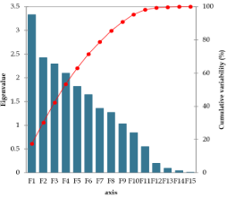
Figure 1. Scree plot of parameters.
Adding more components (F7–F15) contributes little to the cumulative variability (flattened curve).
Based on the screen plot, retaining the first 6 components (F1–F6) is a reasonable choice, as they capture most of the variance while reducing the dimensionality of the dataset. Components beyond F6 (with eigenvalues <1) have a negligible contribution to the variance and can be excluded for simpler and more efficient analysis. This plot highlights how PCA can simplify complex datasets while preserving the most critical information. This figure is a biplot with bootstrap ellipses for the first two principal components (F1 and F2) in a Principal Component Analysis (PCA) (Figure 2). It provides insights into the variability and clustering of observations within the dataset. The horizontal axis (F1) explains 17.53% of the total variance. The first few components (F1 to F6) have the highest eigenvalues and explain most of the variance. After F6, eigenvalues drop below 1, suggesting those components contribute minimally to the total variance. The curve begins to flatten after F6, meaning additional components (e.g., F7–F15) contribute less to explaining the variance. This is often referred to as the elbow point, where the number of components to retain can be decided. F1 through F6 explain approximately 70% – 75% of the total variance, making them sufficient for summarizing the data.
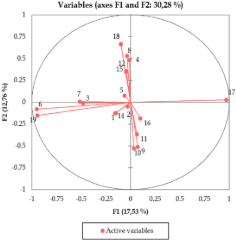
Figure 2. Variables on axes F1 and F2.
The vertical axis (F2) explains 12.76% of the total variance. Together, these two dimensions explain 30.28% of the variability in the data (Figure 3). Each ellipse represents the variability or confidence region of an observation after resampling (bootstrap) (Figure 4). The size of an ellipse indicates the variability in the principal component space. Larger ellipses represent greater uncertainty or variability. Smaller ellipses indicate more stable or consistent observations. Observations such as Obs13 and Obs54 have relatively large ellipses, suggesting higher variability or distinct characteristics in their data. Most observations are clustered near the origin (0, 0), indicating minimal variation along F1 and F2 for these points. Outliers, such as Obs13 and Obs54, are farther from the center, suggesting they are significantly different from the main cluster (Figure 3). The variance explained by F1 and F2 is relatively low (30.28%), meaning additional principal components (e.g., F3, F4) may contribute to capturing more variability in the dataset. Obs13 and Obs54 are distinct observations based on their location and the size of their ellipses. These may warrant further investigation to understand their unique properties or potential data issues.
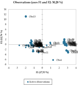
Figure 3. Observations on F1 and F2.
The figure provides insights into data structure and helps identify clusters and outliers. Obs13 and Obs54 may represent distinct groups or anomalies and should be further analyzed. The moderate variance explained (30.28%) suggests that while F1 and F2 capture some key patterns, additional components may be necessary for a comprehensive understanding of the data. This plot is useful for visualizing the relationships among observations and identifying variability or grouping patterns in the data.
The horizontal axis (F1) explains 17.53% of the variance. The vertical axis (F2) explains 12.76% of the variance. Together, these two components account for 30.28% of the total variability in the dataset. While this captures some variability, additional components (e.g., F3, F4) likely hold significant information.
The blue points represent individual observations in the dataset. Most observations are clustered near the origin (0, 0), suggesting they exhibit average characteristics along F1 and F2. Outliers such as Obs13 and Obs54 are located farther from the center, indicating that these observations have distinct patterns or characteristics relative to the majority. The red arrows represent the variables included in the PCA. The direction and length of each arrow indicate direction, i.e. variables pointing in similar directions are positively correlated. The Length, i.e. longer arrows indicate stronger contributions to the variance explained by F1 and F2. Variables pointing in opposite directions have negative correlations.
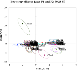
Figure 4. Bootstrap ellipses on axes F1 and F2.
Observations located in the direction of a variable (red arrow) are strongly influenced by that variable. For example, Obs13 aligns more with certain variables, making it distinct from the central cluster. Obs13 and Obs54 are far from the main group and may represent unique patterns or potential anomalies. These could warrant further investigation to understand their significance. Observations closer to the arrows are more influenced by the corresponding variables. Variables pointing toward different quadrants suggest distinct influences on observations. The figure highlights variability among observations and their relationships to variables. Outliers such as Obs13 and Obs54 may represent unique cases worth exploring further. The low variance explained (30.28%) by F1 and F2 suggests that higher components (e.g., F3, F4) should also be examined for a fuller understanding of the dataset. This biplot is a powerful visualization for identifying relationships between observations and variables while highlighting patterns and outliers in the data (Figure 5). Figure 6 is a dendrogram, which is a hierarchical clustering diagram. It visualizes the grouping (clustering) of variables or observations based on their similarity or dissimilarity. The vertical axis represents the dissimilarity or distance between clusters. Higher values indicate greater dissimilarity between groups. The observations or variables are grouped together at different levels of dissimilarity. Clusters are joined at different heights depending on their similarity, with smaller distances (closer to the bottom) indicating more similar observations. This line indicates the threshold or cutoff for grouping.
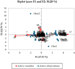
Figure 5. Biplot on Axes F1 and F2.
Observations joined above this line are grouped into distinct clusters. In this case, two main clusters are identified based on the cutoff: C1 (red) and C2 (blue). Contains a large group of closely related observations, as indicated by the shorter branch lengths (lower dissimilarity). This cluster represents observations that are more similar to each other. Contains a smaller group of observations that are distinct from those in C1. The longer branch length leading to C2 suggests that these observations are more dissimilar from those in C1.
The dendrogram helps identify groups of observations with shared characteristics. C1 (Red) likely represents a more homogeneous set of observations, while C2 (Blue) includes outliers or distinct patterns.
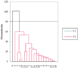
Figure 6. Dendogram.
The cutoff line determines the number of clusters formed. Adjusting this line can result in more or fewer clusters, depending on the level of granularity needed for the analysis. Further analysis of the clusters (e.g., examining their characteristics or performing statistical tests) can provide deeper insights into what differentiates these groups. This dendrogram shows two main clusters (C1 and C2) based on the dissimilarity threshold. C1 contains a larger, more homogeneous group, while C2 includes more distinct or outlier observations. The dendrogram provides a useful way to visualize relationships and structure within the data.
This table represents factor loadings from a Principal Component Analysis (PCA). Factor loadings measure the correlation between the original variables (parameters) and the extracted components (F1–F5). Each parameter's loading shows its contribution to a specific component, with higher absolute values indicating stronger influence. Number of grazing area 1 hectare (P17) is 0.970. The most significant positive contributor, indicating that grazing area (1 hectare) strongly aligns with F1. Number of grazing area 3 hectares (P19) is -0.945. It means that a strong negative contributor, contrasting with 1-hectare grazing. Natural mating (P6) (-0.951) has a strong negative influence on this component. F1 is likely associated with grazing area usage and mating strategies, with contrasting patterns between smaller grazing areas and traditional mating systems. Household Waste (P13) (0.663) and Number of grazing area 2 hectares (P18) is 0.663 showing strong positive contributions. Without Shelter (P8) (0.531) is also a significant positive influence. With Shelter (P9) (-0.510) and Shelter and Free Range (P10) is -0.531 means a negative contribution, contrasting with "Without Shelter. F2 likely reflects feeding systems and sheltering practices, highlighting the influence of feeding types (e.g., household waste) and housing strategies. Number of Offspring per Mother (P1) (0.639) and Births per Mother/Year (P2) (0.642): Strong positive contributors, emphasizing reproductive performance. Without Shelter (P8) (0.535) and Shelter and Free Range (P10) (-0.535): Shelter practices also influence F3. F3 represents reproductive productivity and sheltering systems, indicating a link between sheltering conditions and breeding success.
Commercial Feed (P11) (0.514) and With Shelter (P9) (0.509): Strong positive contributors. Household Waste (P13) (0.495): Another significant positive influence. F4 likely reflects feeding and shelter efficiency, particularly the impact of commercial feed and household waste on livestock performance. Without Shelter (P8) (0.625), Commercial Feed (P11) (0.626), and With Shelter (P9) (0.420): Strong positive contributors. Shelter and Free Range (P10) (-0.625): A strong negative influence, contrasting with structured shelter systems. F5 captures contrasting housing and feeding strategies, differentiating structured shelter and feed systems from mixed or free-range systems.
Number of offspring per parent (P1) and Births per parent/Year (P2) strongly influence F3, empha-sizing their role in breeding efficiency. One hectare grazing (P17) dominates F1, contrasting with 3 hectares grazing (P19). The F1 highlights the effect of grazing area size on livestock systems. Shelter variables (P8, P9, P10) contribute significantly across F2, F3, and F5, indicating their central role in livestock management. Commercial Feed (P11) and Household Waste (P13) influence F4 and F5, suggesting their impact on efficiency and livestock performance. This analysis highlights the distinct roles of grazing areas, feeding types, breeding productivity, and shelter systems in shaping livestock management outcomes.
4. Conclusions
Conclusions of this study constitute traditional practices dominate in terms of breeding, feeding, and management systems, with limited adoption of modern techniques or infrastructure. The number of offspring or parent, births/parent/year, mating system, management system, feed type, and feeding frequency (specifically once a day) are significant factors influencing livestock outcomes. Wild livestock, natural mating, and artificial insemination significantly impact livestock performance.
Acknowledgements
The authors sincerely thank the livestock farmers in Manokwari Regency, West Papua, for their cooperation and willingness to share information during field data collection. Appreciation is also extended to local agricultural and livestock officers for their logistical support and valuable insights during the research process. The authors gratefully acknowledge all individuals who contributed to this study but are not listed as co-authors.
Conflict of Interest
The authors declare that there is no conflict of interest regarding the publication of this manuscript.
Funding Statement
This research did not receive any specific grant from funding agencies in the public, commercial, or not-for-profit sectors.
References
Argo, A., Rahardjo, K., & Wicaksono, K. P. (2015). Optimalisasi Strategi Integrasi Kelapa Sawit-Sapi Pada Badan Usaha Milik Negara (BUMN) Perkebunan Di Indonesia. Profit, 9(1), 11–21. https://doi.org/10.21776/ub.profit.2015.009.01.2
Bolowe, M. A., Ketshephaone, T., Monametsi, P., Ineeleng, P., & Malejane, C. (2022). Production Characteristics and Management Practices of Indigenous Tswana Sheep in Southern Districts of Botswana. Animals, 12(7), 830. https://doi.org/10.3390/ani12070830
Boujenane, I. (2015). Growth at Fattening and Carcass Characteristics of D’man, Sardi and Meat-Sire Crossbred Lambs Slaughtered at Two Stages of Maturity. Tropical Animal Health and Production, 47(7), 1363–71. https://doi.org/10.1007/s11250-015-0872-x
Clough, Y., Vijesh, V. K., Corre, M. D., Darras, K., Denmead, L. H., Meijide, A., Moser, S., et al. (2016). Land-Use Choices Follow Profitability at the Expense of Ecological Functions in Indonesian Smallholder Landscapes. Nature Communications, 7. https://doi.org/10.1038/ncomms13137
Creswell, J. W. (2014). Research Design: Qualitative, Quantitative, and Mixed Methods Approaches. SAGE Publications.
Das, G. (2018). Traditional Livestock Management of the Tribal Communities in the State of Andhra Pradesh and Telangana. Tarnaka Secunderabad India.
Descheemaeker, K., Amede, T., & Haileslassie, A. (2010). Improving Water Productivity in Mixed Crop-Livestock Farming Systems of Sub-Saharan Africa. Agricultural Water Management, 97(5), 579–86. https://doi.org/10.1016/j.agwat.2009.11.012
Fanimo, A. O., Oduguwa, O. O., Adesehinwa, A. O. K., Owoeye, E. Y., & Babatunde, O. S. (2003). Response of Weaner Pigs to Feed Rationing and Frequency of Feeding. Livestock Research for Rural Development,15(6), 26–30.
Far, Z., & Yakhler, H. (2015). Typology of Cattle Farming Systems in the Semi-Arid Region of Setif: Diversity of Productive Directions? Livestock Research for Rural Development, 27(6).
Frison, E. A., Cherfas, J., & Hodgkin, T. (2011). Agricultural Biodiversity Is Essential for a Sustainable Improvement in Food and Nutrition Security. Sustainability, 3(1), 238–53. https://doi.org/10.3390/su3010238
Gizaw, S., Getachew, T., Goshme, S., Valle-Zárate, A., Van Arendonk, J. A. M., Kemp, S., Mwai, A. O., & Dessie, T. (2014). Efficiency of Selection for Body Weight in a Cooperative Village Breeding Program of Menz Sheep under Smallholder Farming System. Animal, 8(8), 1249–54. https://doi.org/10.1017/S1751731113002024
Goddard, M. A., Dougill, A. J., & Benton, T. G. (2013). Why Garden for Wildlife? Social and Ecological Drivers, Motivations and Barriers for Biodiversity Management in Residential Landscapes. Ecological Economics, 86, 258–73. https://doi.org/10.1016/j.ecolecon.2012.07.016.
Hosseini, M., Shahrbabak, H. M., Zandi, M. B., & Fallahi, M. H. (2016). A Morphometric Survey among Three Iranian Horse Breeds with Multivariate Analysis. Media Peternakan, 39(3), 155–60. https://doi.org/10.5398/medpet.2016.39.3.155
Hutabarat, S. (2017). Rakyat Di Kabupaten Pelalawan, Riau Dalam Perubahan Perdagangan Global. Pekanbaru Indonesia, 43, 47–64.
Iyai, D. A., Rahayu, B. W. I., Sumpe, I., & Saragih, D. (2011). Analysis of Pig Profiles on Small-Scale Pig Farmers in Manokwari-West Papua. Journal of the Indonesian Tropical Animal Agriculture, 36 (3), 190–197. https://doi.org/10.14710/jitaa.36.3.190-197
Iyai, D., Mustaqim, A. I., & Sagrim, M. (2020). Profil, Input Dan Output Sistem Peternakan Pada Kawasan Agro-Ekologi Tambrauw Provinsi Papua Barat. Jurnal Pertanian Terpadu, 8(1), 1–13. https://doi.org/10.36084/jpt..v8i1.230
Kamau, P. (2004). Forage Diversity and Impact of Grazing Management on Rangeland Ecosystems in Mbeere District, Kenya. Kenya.
Manokwari, B. P. S. (2018). Kabupaten Manokwari Dalam Angka 2018. Manokwari: BPS Manokwari.
Marandure, T., Dzama, K., Bennett, J., Makombe, G., Chikwanha, O., & Mapiye, C. (2020). Farmer Challenge-Derived Indicators for Assessing Sustainability of Low-Input Ruminant Production Systems in Sub-Saharan Africa. Environmental and Sustainability Indicators, 8(August), 100060. https://doi.org/10.1016/j.indic.2020.100060
Marie, D., Nkou, B. B., Voundi, E., Ghazoul, J., Mala, A. W., Buttler, A., & Guillaume, T. (2023). Nutrient Availability Challenges the Sustainability of Low-Input Oil Palm Farming Systems. Farming System, 1(1), 100006. https://doi.org/10.1016/j.farsys.2023.100006
McCarthy, J. F. (2010). Processes of Inclusion and Adverse Incorporation: Oil Palm and Agrarian Change in Sumatra, Indonesia. Journal of Peasant Studies, 37(4), 821–50. https://doi.org/10.1080/03066150.2010.512460
Mekonnen, A., Haile, A., Dessie, T., & Mekasha, Y. (2012). On Farm Characterization of Horro Cattle Breed Production Systems in Western Oromia, Ethiopia. Livestock Research for Rural Development, 24(6), 7.
Mezgebe, G., Gizaw, S., & Urge, M. (2018). Economic Values of Begait Cattle Breeding-Objective Traits under Low and Medium Input Production Systems in Northern Ethiopia. Livestock Research for Rural Development, 30(1).
Muhlisin, P., Lee, S. J., Lee, J. K., & Lee, S. K. (2014). Effects of Crossbreeding and Gender on the Carcass Traits and Meat Quality of Korean Native Black Pig and Duroc Crossbred. Asian-Australasian Journal of Animal Sciences, 27(7), 1019–1025. https://doi.org/10.5713/ajas.2013.13734
Musa, M. A., Peters, K. J., & Ahmed, M. K. A. (2006). On Farm Characterization of Butana and Kenana Cattle Breed Production Systems in Sudan. Livestock Research for Rural Development, 18(12).
Pagala, M. A., Zulkarnain, D., & Munadi, L. M. (2020). Kapasitas Daya Tampung Hijauan Pakan Ternak Dan Hasil Ikutan Perkebunan Kelapa Sawit Di Kecamatan Tanggetada Kabupaten Kolaka. Jurnal Sosio Agribisnis, 5(2), 70–76.
Parsons, D., Lane, P. A., Ngoan, L. D., Ba, N. X., Tuan, D. T., Van, N. H., Dung, D. V., & Phung, L. D. (2013). Systems of Cattle Production in South Central Coastal Vietnam. Livestock Research for Rural Development, 25(2).
Pasandaran, E. (2006). Alternative Policies for Controlling Conversion of Irrigated Rice Fields in Indonesia. Jurnal Litbang Pertanian, 25(4), 123–129.
Pattiselanno, F., Desni, T. R., Saragih, M., Lekitoo, N., & Iyai, D. A. (2021). Nutrient Values of Utilization of Crops Wastes as Alternative Pig Feeding Ingredient in The Coastal Agro-Ecological Area of Manokwari, West Papua. Jurnal Ilmiah Peternakan Terpadu, 9(2), 170. https://doi.org/10.23960/jipt.v9i2.p170-185
Petrus, N. P., Mpofu, I., Schneider, M. B., & Nepembe, M. (2011). The Constraints and Potentials of Pig Production among Communal Farmers in Etayi Constituency of Namibia. Livestock Research for Rural Development, 23(7), 18125.
Rao, G. N. (2018). Biostatistics & Research Methodology. PharmaMed Press.
Rojas-Downing, M., Melissa, A., Nejadhashemi, P., Harrigan, T., & Woznicki, S. A. (2017). Climate Change and Livestock: Impacts, Adaptation, and Mitigation. Climate Risk Management, 16, 145–163. https://doi.org/10.1016/j.crm.2017.02.001
Sayori, A., Widayati, T. W., Supriyantono, A., Randa, S. Y., & Iyai, D. A. (2022). Pig Farming System in West Papua: A Case Study of Three Districts. Annals of Agriculture Science and Research, 1(1), 1–10.
Serey, M., Mom, S., Kouch, T., & Bunna, C. (2014). Cattle Production Systems in NW Cambodia. Livestock Research for Rural Development, 26(3), 86320.
Shikuku, K. M., Valdivia, R. O., Paul, B. K., Mwongera, C., Winowiecki, L., Läderach, P., Herrero, M., & Silvestri, S. (2017). Prioritizing Climate-Smart Livestock Technologies in Rural Tanzania: A Minimum Data Approach. Agricultural Systems, 151, 204–216. https://doi.org/10.1016/j.agsy.2016.06.004
Sibly, R. M., Grimm, V., Martin, B. T., Johnston, A. S. A., Kulakowska, K., Topping, C. J., Calow, P., Nabe-Nielsen, J., Thorbek, P., & Deangelis, D. L. (2013). Representing the Acquisition and Use of Energy by Individuals in Agent-Based Models of Animal Populations. Methods in Ecology and Evolution, 4(2), 151–161. https://doi.org/10.1111/2041-210x.12002
Snedecor, G. W., & Cochran, W. G. (1989). Statistical Methods. 8th ed. USA: Blackwell Publishing.
Solomon, Z. A., Kassa, B., Agza, B., Alemu, F., & Muleta, G. (2014). Smallholder Cattle Production Systems in Metekel Zone, Northwest Ethiopia. Research Journal of Agriculture and Environmental Management, 3(2), 151–157.
Steffens, V. C. (2016). Potentials of Agrarian Cluster Development for Improving Smallholder ’ s Income – a Case Study from the SAGCOT Initiative in Tanzania. Universität zu Köln.
Tohiran, K. A., Nobilly, F., Zulkifli, R., Ashton-Butt, A., & Azhar, B. (2019). Cattle-Grazing in Oil Palm Plantations Sustainably Controls Understory Vegetation. Agriculture, Ecosystems and Environment, 278(March), 54–60. https://doi.org/10.1016/j.agee.2019.03.021.
Tolera, A., & Abebe, A. (2007). Livestock Production in Pastoral and Agro-Pastoral Production Systems of Southern Ethiopia. Livestock Research for Rural Development, 19(12), 2007.
Winarso, B., & Basuno, E. (2013). Pengembangan Pola Integrasi Tanaman-Ternak Merupakan Bagian Upaya Mendukung Usaha Pembibitan Sapi Potong Dalam Negeri. Forum Penelitian Agro Ekonomi, 31(2), 151. https://doi.org/10.21082/fae.v31n2.2013.151-169